GEOG 581: Cartography Design

Customize Topography and 3D representation

LAB-3, created by Dr. Tsou, 10 points

 Many thanks to Dr. Ailleen Buckley from ESRI. for her generous help in providing the materials and tools for this lab exercises.

First of all, let's create a folder called "Lab-03" in your own course folder at the Z: drive.

Open ArcMap with a new empty map.

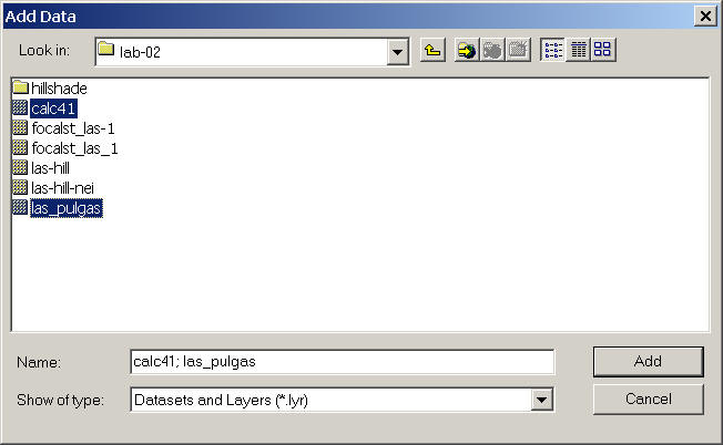
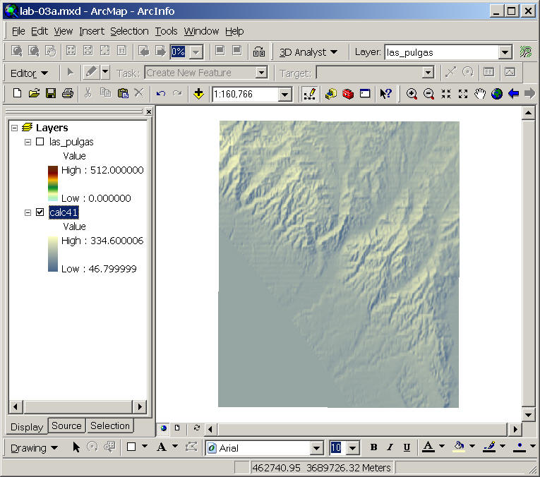
Add two layers (original DEM GRID (the location name) and the calculated hillshade (calc42) from the "lab-02" folder, last week).

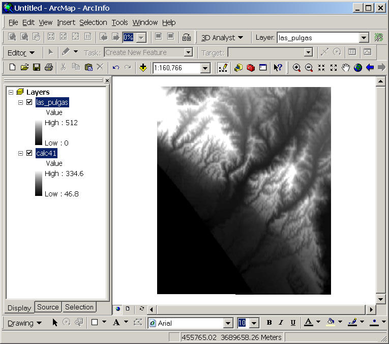
Change the dem layer with elevation#1 color ramp. 

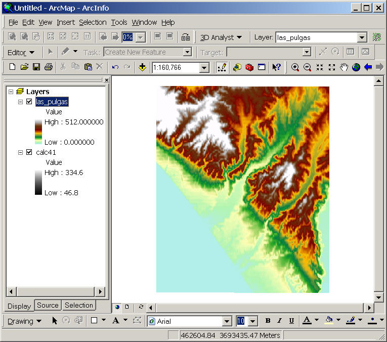
Now the problem is that we can see the "white snow" on the top of mountain.  But in San Diego, we usually don't have snow!   To correct this, open the DEM layer property window again and right click on the  Color Ramp and then select "Properties"

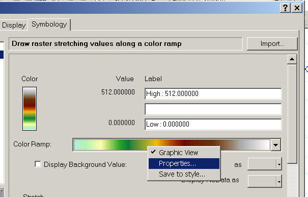
Select the bottom two layers and "Remove" them (one by one).  Then click on [OK]

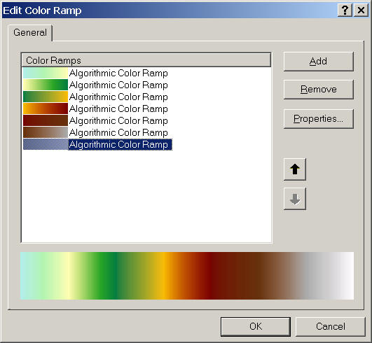
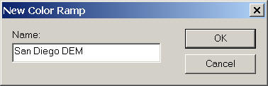
Now right click on the color ramp again and select "Save to Style".  Type San Diego DEM for the Name and click OK.

Now you can see the white snow mountain disappear.

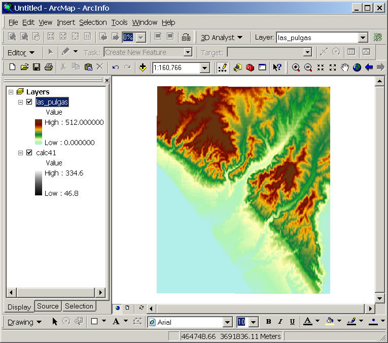
Now change the transparency of this DEM to 35%.  Our next step is to create another effect for hillshade.

Open the layer property of hillshade (calc42) and select symbology.  We will change the color ramp to a blue to yellow ramp which simulates sunshine on surfaces toward the light and blue shadows in areas that are less illuminated.

Go to Tools menu --> Styles --> Style Reference.

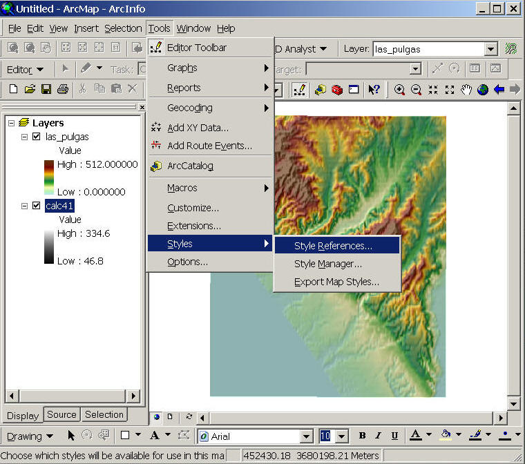
Click on "Add"---> Navigate to Z:\data\style --> select Elevation.style.  click [O.K] to continue.

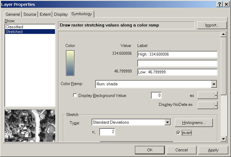
Uncheck the DEM layer now.  Then open the Calc42 layer property window.

In the symbology tab, Select "Illum. Shade" from the Color Ramp list.  Also, check the "Invert" box to switch the color of yellow and blue. Click on O.K.

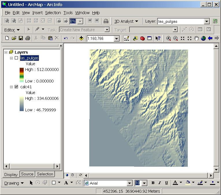
Let's see the original illuminated effect.  Did you feel the sunshine on the mountain?

Now, open the "calc42" property window.

Change the stretch type to "None".  Then OK.

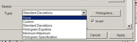
Now, this is a smoother hillshade effect...

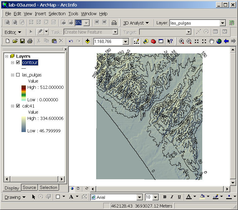
Save your map into lab-03 folder as "lab-03a.mxd"

Variable Depth Masking

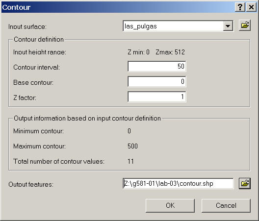
First, let's create a contour line from the 3D analyst. --> select [3D Analyst] --> Surface Analysis --> Contour.  (remember to turn on the 3D analyst extension and the tool bar --- refer to the first week exercises).

Change the Contour interval to 50. (Please feel free to change this number according to your own situation.  Some DEMs needs more, some needs less).  Also, change the Output features to Z:\g581-##(your folder)\lab-03\contour.shp.

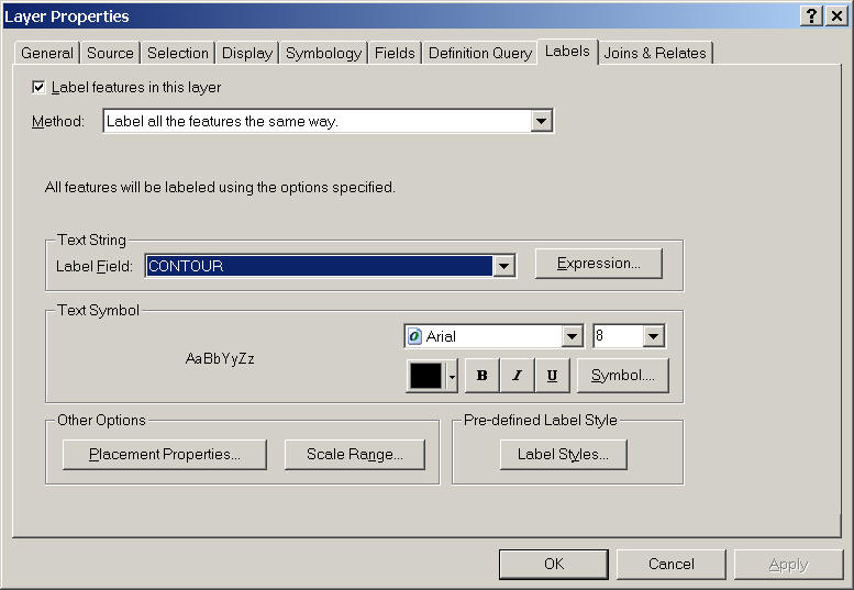
Open the contour layer's properties.  Check the label features... box.   Select "CONTOUR" in the Label Field.  Click on OK to apply.

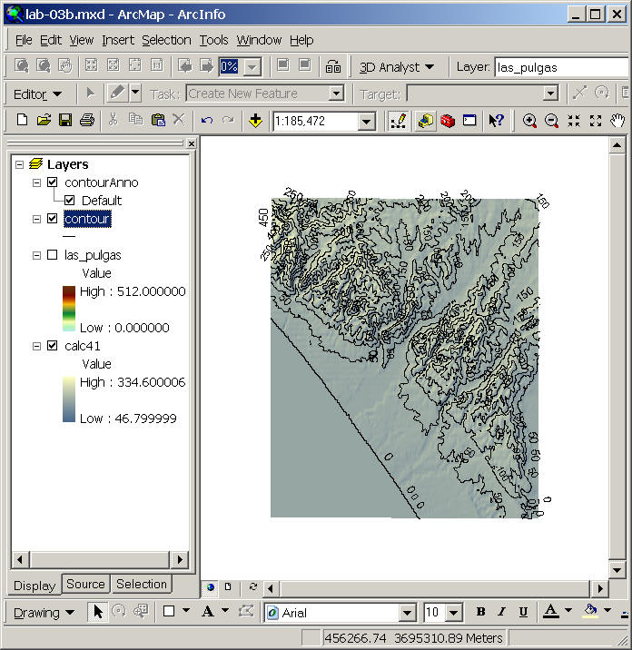
Now we created a contours.  However, it is very mixed and difficult to recognize.

To create a variable depth masking, the first step is to convert labels to annotation. 

Please use ArcGIS help to compare the differences between labels and annotations.

The first thing is to create a Geodatabases to store our annotation.

(Use online HELP to learn what is geodatabases..)

Open the ArcCatalog first (from ArcMap). Navigate to "lab-03" folder.  Select File --> New --> Personal Geodatabase

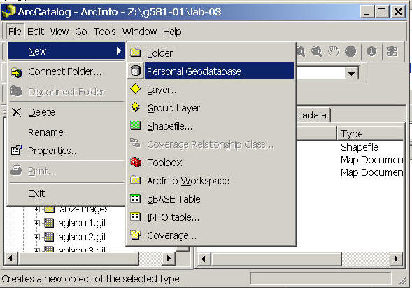
Change the name to "lab-03.mdb".

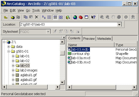
Close the ArcCatalog.

Now back to ArcMap. Right click the contour layer and select "convert labels to annotation".

Use the default setting, (Store Annotation In a database)..  click on the yellow folder icon to navigate to the "Lab-03.mdb" file we just create.  (Click on Save  -->  then "Convert")

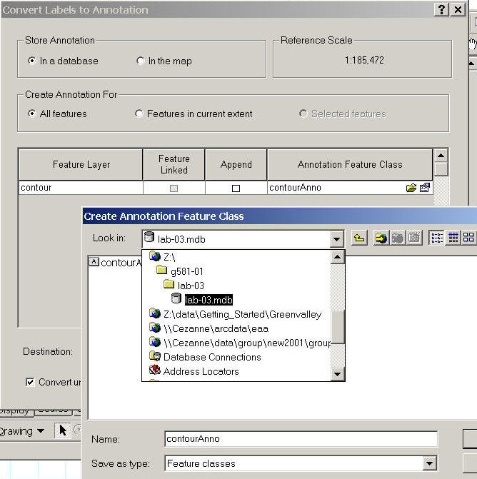
After the process,  a new layer (contourAnno) will show up on ArcMap.

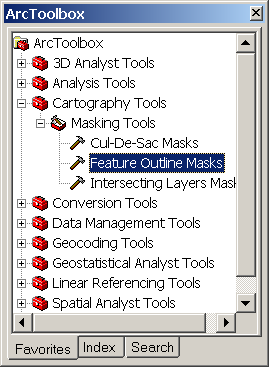
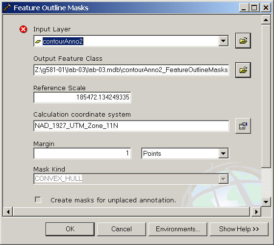
Next step is to open ArcToolbox.  Select Cartography Tools --> Feature Outline Masks.

Select the contourAnno as Input layer, change the Margin to "1" points. "Uncheck the box for "create masks for unplaced anotation".

Click on OK.

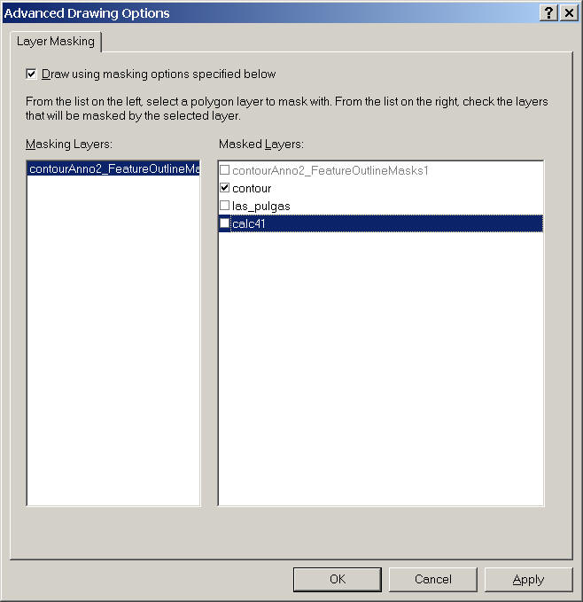
Right click on the "Layer" frame, then select "Advanced Drawing Options".

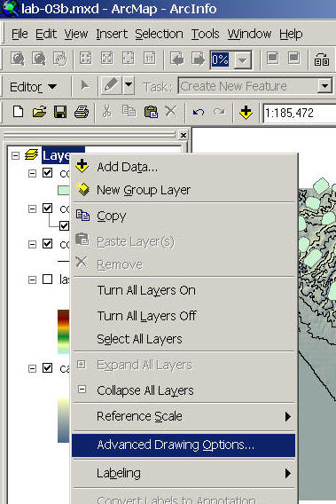
Check the box for "Draw using masking options.  Then select "contour" as the masked layer.

Click on OK.

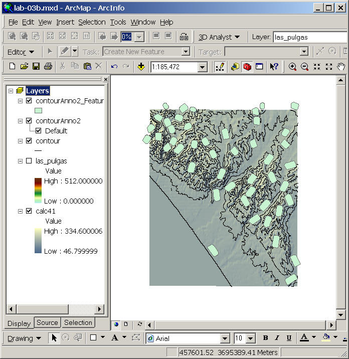
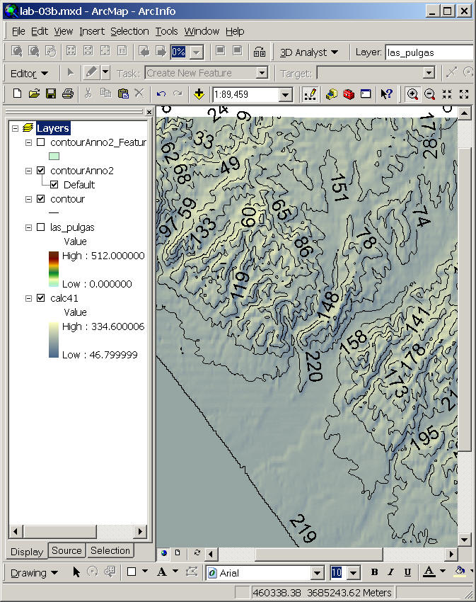
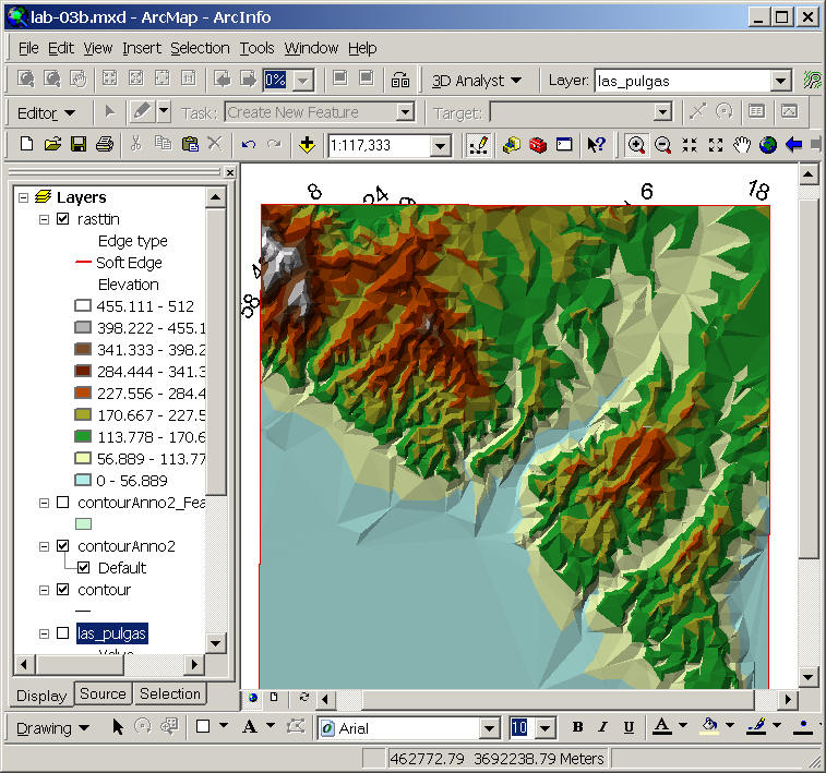
Now uncheck the contourAnnoFeature layer (the first one).  You will see the label of contour line is clearly display on your ArcMap (with masked contour line).

O.K.  now save as your map into the lab-03 folder as lab-03b.mdb.

3D Display

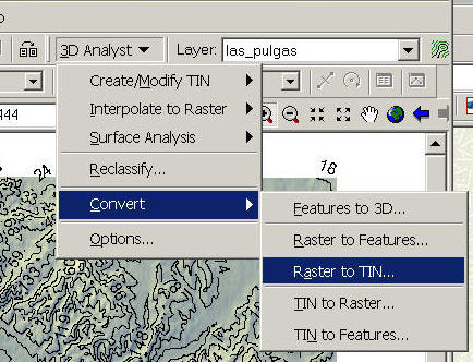
The first step is to create a TIN model.  Select 3D Analyst --> Convert --> Raster to TIN

(make sure the input file is the orginal DEM file).

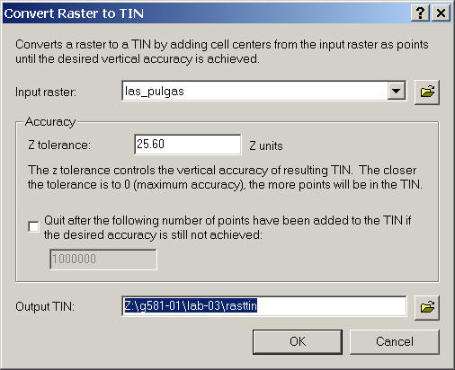
Save as your ArcMap to "lab-03" folder as lab-03c.mxd.

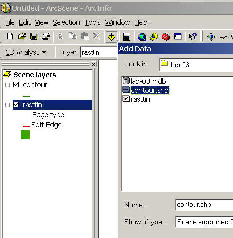
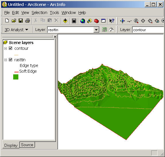
Now from the 3D Analyst menu, click on the yellow ArcScene icon.

From the ArcScene, click on Add data icon and add contour and rastin layer into ArcScene.

Try to move the 3D view and familiar with the functions in ArcScene (very similar to ArcGlobe.)

Double click on the "Rastin" to open the layer properties, select "Base Heights" and change the Z unit to "5".

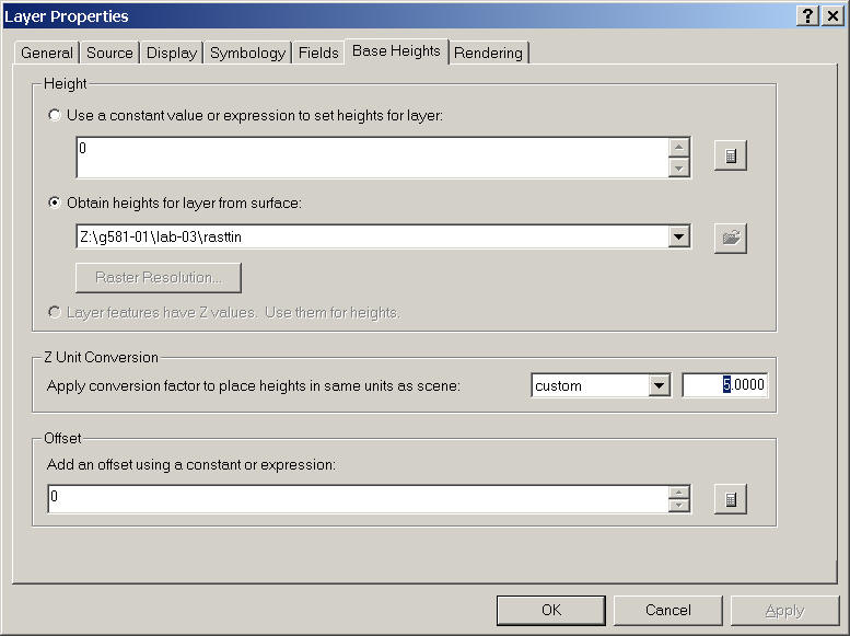
Now you can see the terrain has been exaggerated a little.

Open the contour layer property, open the Base Height, --> select "Obtain heights from layer...

Change the Z unit also to "5".   click OK.

(Try to find out what is Z unit? what is Offset? from on-line help)

Now you can see the contour line is draped into the 3D terrain.

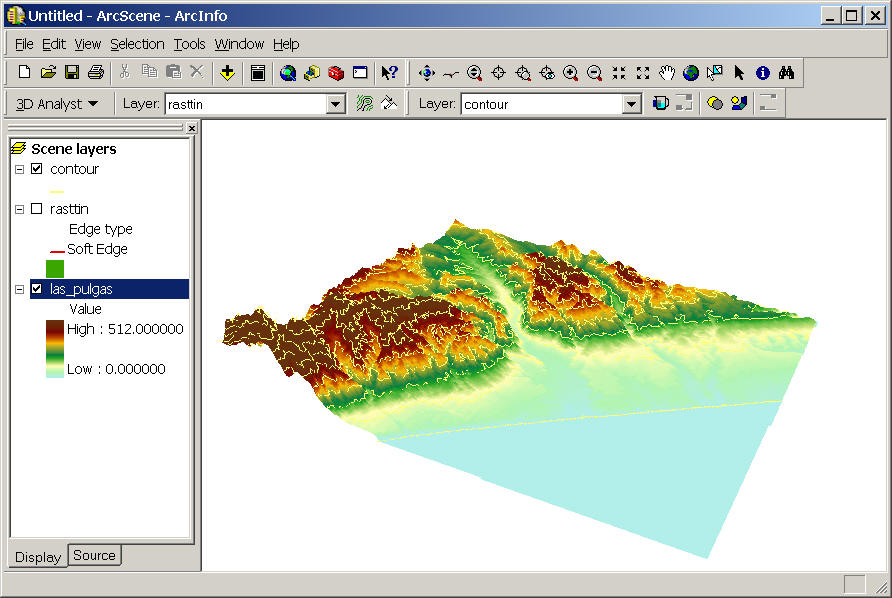
Now try to add the original DEM into the ArcScene.

(DEM is from lab-02 folder.  You can also uncheck the rasttin for the display. 

Save the ArcScene to lab-03 folder as lab-03.sxd.

Close the ArcScene and ArcMap.

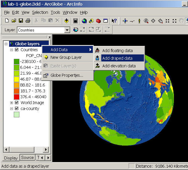
Now launch the ArcGloble from the Program menu.

Open your first lab-1-globe.3dd from the "Lab-01" folder. (the file you saved in lab one).

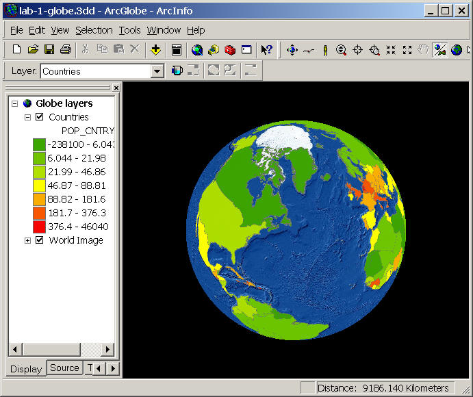
First of all, right click on the "Globe layer" select "add draped data"

Navigate to Z:\data\ca\  select ca-county.shp.

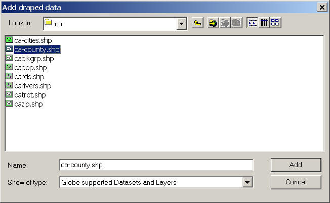
(Use Help to find out what's the differences between floating data, draped data, and elevation data.)

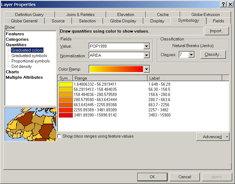
Modify the symbols for CA-county and display the population density in 1999 (refer to the lab-1 for details).

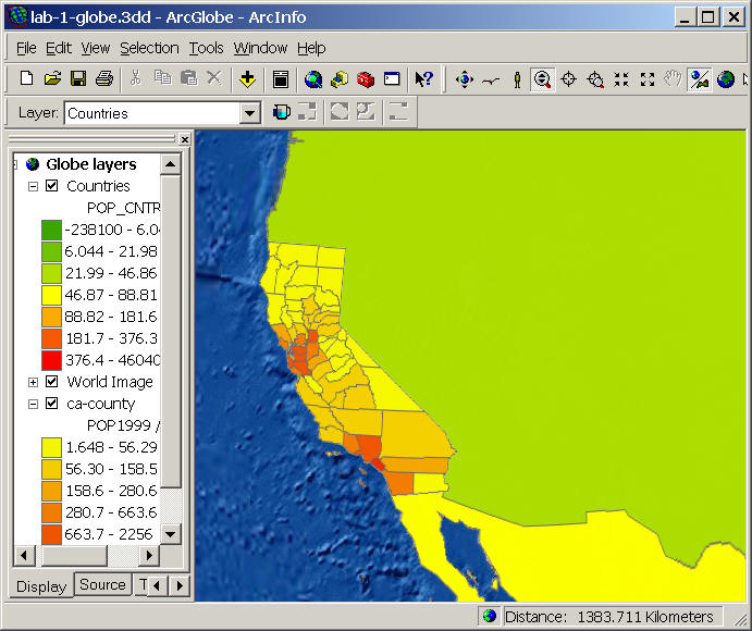
Now try to zoom in to see the California State from the ArcGloble.

Now right click on the Globe layers, --> Add data --> add "elevation data"

Select lab-02  your original DEM elevation

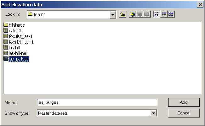
Next, add another draped data to ArcGlable from lab-02 "Calc41"

Use the navigation tools to change the view as the following:

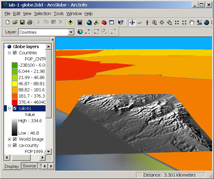
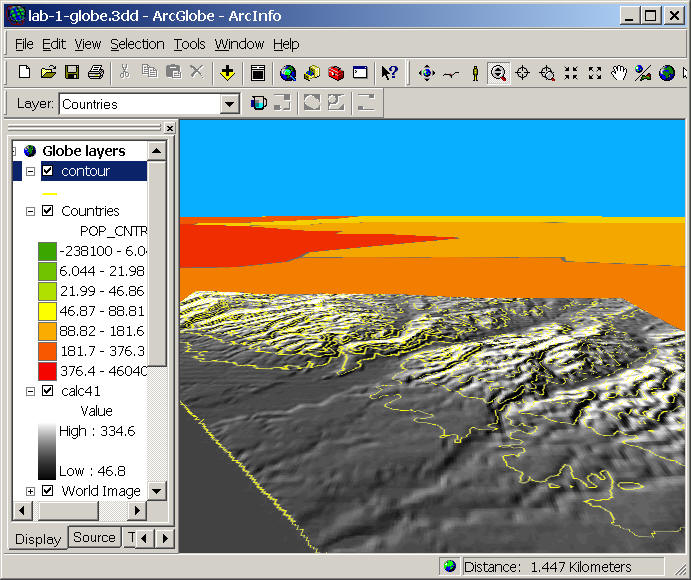
Then add the contour line from the lab-03 folder. set the line color to yellow

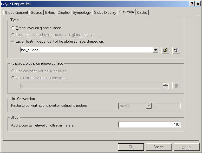
Now the view is still not a 3D terrain.  To change that open the layer property for Calc42.

Select "layer floats .... with the orignal DEM file. and Offset as 100.

Do the same thing for the contour line. but set the offset as 120.

Now the terrain looks better.

Now try to add more GIS layers into the ArcGlobe, and give appropriate setting and color scheme for each. (like Aspects, rivers. schools,.etc.)

Our next step is to create a short movie to navigate from Space to San Diego.

Switch back to the Global view.

Select View --> Toolbars --> Animation.

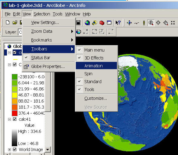
Click on the  "open animation controls" icon (next to the camera icon).

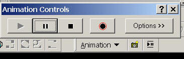
Try to create an animation from globe to california to San Diego.

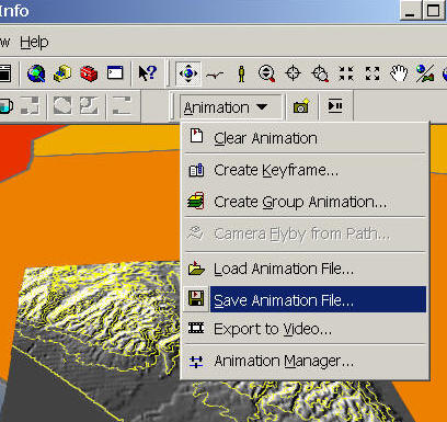
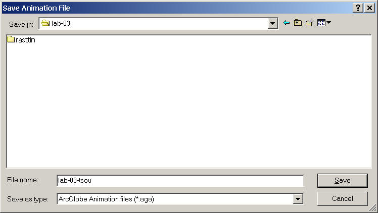
Save your animation file into "lab-03" folder as lab-03-yourlastname.aga.

When you finish, save your ArcGlobe file into "lab-03" folder as "lab-3-globle.3dd."

Now we are all done for today's lab.  

Prepare to share your animation to other class members next time.

Your animation will have 5 points for this lab.

Note: If your computer is too slow in ArcGloble, you can try to copy all the data (lab-02, lab-03, CA folders) into a local C:\temp folder.  The response may be faster.  But since you save these data into the local folder.  If you change the machine next time, you will not be able to see your animation.  To solve the problem, you can export your animation to AVI or MOV files.