Web-based Exercise #6:

1.     Overview

Grading:  8 points total.

Learning Goal:  This exercise will introduce basic concepts of Geovisualization and spatial statistical analysis. After finishing this exercise, the students should be able to learn the most common spatial data analysis techniques in the context of exploratory data analysis environment.

Platforms:  PC, Mac, or UNIX.  Please make sure the JRE (Java Runtime Environment) has been successfully installed in your computer.

Due Day: (SKIP in Fall 2013)

You should upload your lab answers to the Blackboard ( http://blackboard.sdsu.edu )  before the lecture and submit a paper print-out version in the class.  We will use the Timestamp on your documents in the Blackboard to check if your assignment is late or not.

(In your upload file, please use this title: [GEOG104-LAB-6-[Your name].doc (or txt or pdf).  Please write down your answers in MS Word or WordPAD or other word processing software.  Please always save a local backup copy of your own answers.)

If you don't have Internet access, you can use our SAL lab (Storm Hall 338, third floor) on every Friday morning from 11:00am to 12:00pm.

 

2.     Web-based Analytical Tools at SAL (Spatial Analysis Laboratory), UIUC

Dr. Luc Anselin, the director of the GeoDa Center at UIUC, has been working on the development of theories and computer-based tools for spatial statistics for several decades. As one of his major contribution, GeoDa (http://geodacenter.asu.edu/) is a typical spatial statistical analysis package devoted to the discovery of spatial patterns embedded in the geographical data.

Please visit the GeoData Center web pages (http://geodacenter.asu.edu/).

 

Answer question Q1 (please use Web search engine for more information or review http://en.wikipedia.org/wiki/Spatial_analysis,  and http://biosun1.harvard.edu/research/divisions/env_stat/GISinLMA/spatstat.htm).

Q1: What is spatial statistics? What are the differences between spatial statistics and the general statistics, or in other words, what makes spatial statistics special?

 

In this exercise, we will examine a simple web-based spatial analysis tool or so called, "Web-based Tools Project". Click this hyperlink: http://geodacenter.asu.edu/webesda_overview  or you can access this web page from the "Projects" menu  (Figure 1).

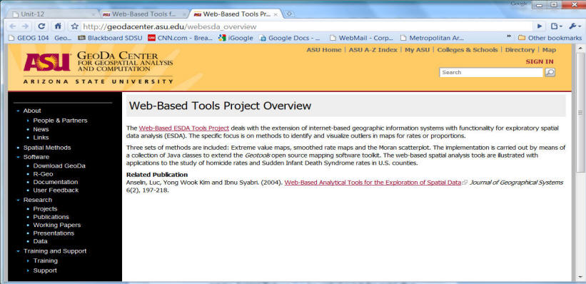
       Figure 1. The web page for the web-based ESDA project

 

Web-Based Analytical Tools for the Exploration of Spatial Data Journal of Geographical Systems6(2), 197-218.

    Figure 2. The web page for the web-based spatial statistical tools

From the web page, select the screen resolution, the dataset (here we use “St. Louis Ring”), and  “Moran Scatterplot”. Then click on “Create Applet” to start the analysis. For more information about “Moran Scatterplot”, please visit http://www.terraseer.com/products/stis/help/Statistics/LM/Results/Moran_Scatter_Plot.htm.

For the introduction of the dataset “St. Louis Ring”, please refer to research paper “Web-based Analytical Tools for the Exploration of Spatial Data “ (page 13-14).

The figure 3 shows the running Java applet looks.

     Figure 3. The Java Applet for the analysis of St. Louis Ring dataset

Double click the legend. In the pop-up dialog (Figure 4), customize the starting and ending colors, specify the “Category Count”, select the “Event”, the “Base” and the mapping mode.

 Figure 4. The mapping interface

This following map (figure 5) shows an example: describing the event “HC8893” (homicide count between 1988-1993) based on “PO8893” (the entire population for 1988-1993) with category-count -- 3  in the mode of “Excess Rate Map”.

     Figure 5. The Excess Rate Map for the St. Louis Ring dataset

Answer the question Q2.

Q2: What is the excess rate? (refer to research paper “Web-based Analytical Tools for the Exploration of Spatial Data “) From the excess rate map, what county/city has the highest homicide rate? What spatial patterns can be seen from this map? 

(Tip:  When you move the mouse cursor inside a county boundary, the county name will pop-up from the web browser.)

Use the same “Event” and “Base”, however choose “Box Map” as the mapping mode (Figure 6).

        Figure 6. The Box Map for the St. Louis Ring dataset

Choose “EB” (Empirical Bayes) smoothing method and click on the “Smooth” button (Figure 7).

         Figure 7. The Box Map with EB Smoothing for the St. Louis Ring dataset

Answer the question Q3.

Q3: What is the box map? (refer to the definition of box plot in wikipedia: http://en.wikipedia.org/wiki/Box_plot ) Compare the two box maps (one with original raw rate and the other with EB smoothing). What are the differences? Which counties appear to become outliers in the smoothing map? If you want to look at one with original raw rate, click "Reset" button.

Choose another smoothing method “SR” (Spatial Rate) and produce new map (Figure 8).

            Figure 8. The Box Map with SR Smoothing for the St. Louis Ring dataset

Answer the question Q4.

Q4: Compare the spatial smoothing map with the EB smoothing map. Again, what counties become outliers in the spatial smoothing map and why?

When you start the analysis, make sure select “Moran Scatterplot” (in Figure 2).

Click on the “Matrix” button on the top of the map. After building of the spatial weight matrix, click on the “Moransl” button to generate the Moran scatterplot (Figure 9). Notice that the box map and the Moran Scatterplot are linked. Moving the mouse to any unit in the map or the plot can see the corresponding polygons/points being highlighted.

       Figure 9. The Moran Scatterplot for the St. Louis Ring dataset

Answer the question Q5.

Q5: What is the Moran’s I value? (Is it high or low? What does it imply? Try to explain the spatial patterns from the scatterplot from the perspective of spatial autocorrelation (e.g. the clusters of high homicide counts vs. low homicide counts).

Click on the “Subset” button and select a subset of the counties (with selection rectangle) at your will. Recalculate the Moran’s I value. Answer the question Q6.

Q6: What is the Moran’s I value for your subset counties? (Please, capture the subset window including the map and the Moran's I scatterplot, and include it in your answer) Did you include St. Louis City and St. Clair County in your subset? Discuss why the new Moran’s I value is different from the previous one. Any effects by removing the high homicide count outliers such as St. Louis City and St. Clair County?

3.      STARS (Space–Time Analysis of Regional Systems)

As introduced by Dr. Rey in the class, STARS is a spatial-temporal data analysis package. Go to http://regionalanalysislab.org/index.php/Main/STARS for a simple overview of this program. For a more detailed introduction, see the research article written by Dr. Rey and Dr. Janikas (Rey, S.J. and M.V. Janikas (2006) STARS: Space–Time Analysis of Regional Systems, Geographical Analysis 38: 67-84.). You can download it on the campus by clicking http://www3.interscience.wiley.com/cgi-bin/fulltext/118569680/PDFSTART .

 

 

If possible (not required), install STARS in your own computer. The most updated version is 0.8.2. You can obtain it from http://regionalanalysislab.org/?n=Download. Choose the installer according to your operating system. Use the default U.S. dataset (by selecting the menu, “Help”->”Example Project”).

 

Answer the question 7 and 8.

 

Q7: Discuss the importance of visualization in the process of spatial analysis. Use STARS as an example, list the most common Geovisualization methods and discuss their benefits and effects in visualizing the original data and the analysis results?

 

Q8: What are the advantages of web-based spatial data analysis over the traditional desktop tools (e.g. STARS)? What can be improved for the current web-based GIS analysis tools given the SAL web-based ESDA tools as an example? What could be the challenges in migrating the full functions currently implemented in desktop ESDA tools into the web?

 

Web-based Exercise #6:

Spatial Statistics and Analysis.

(SKIP in Fall 2013)

You should upload your lab answers to the Blackboard ( http://blackboard.sdsu.edu )  before the lecture and submit a paper print-out version in the class.  We will use the Timestamp on your documents in the Blackboard to check if your assignment is late or not.

(In your upload file, please use this title: [GEOG104-LAB-#-[Your name].doc (or txt or pdf).  Please write down your answers in MS Word or WordPAD or other word processing software.  Please always save a local backup copy of your own answers.)

Grading:  8 points total

 

Q1: What is spatial statistics? What are the differences between spatial statistics and the general statistics, or in other words, what makes spatial statistics special?

 

Q2: What is the excess rate? (refer to research paper “Web-based Analytical Tools for the Exploration of Spatial Data “) From the excess rate map, what county/city has the highest homicide rate? What spatial patterns can be seen from this map? 

 

Q3: What is the box map? (refer to the definition of box plot in the Wikipedia: http://en.wikipedia.org/wiki/Box_plot ) Compare the two box maps (one with original raw rate and the other with EB smoothing). What are the differences? Which counties appear to become outliers in the smoothing map? If you want to look at one with original raw rate, click "Reset" button.

 

Q4: Compare the spatial smoothing map with the EB smoothing map. Again, what counties become outliers in the spatial smoothing map and why?

 

Q5: What is the Moran’I value? (Is it high or low? What does it imply? Try to explain the spatial patterns from the scatterplot from the perspective of spatial autocorrelation (e.g. the clusters of high homicide counts vs. low homicide counts).

 

Q7: Discuss the importance of visualization in the process of spatial analysis. Use STARS as an example, list the most common Geovisualization methods and discuss their benefits and effects in visualizing the original data and the analysis results?

Q8: What are the advantages of web-based spatial data analysis over the traditional desktop tools (e.g. STARS)? What can be improved for the current web-based GIS analysis tools given the SAL web-based ESDA tools as an example? What could be the challenges in migrating the full functions currently implemented in desktop ESDA tools into the web?